Optimizing astcenc

After two years of incremental improvement the astcenc 3.6 release is around 20 to 25 times faster than the 1.7 release I started with. This blog is a look at some of the techniques I used, and a few that I tried that didn’t work.

The Pareto frontier

Before I dive into details of the software optimization techniques, I need to talk about the the Pareto frontier and how it relates to users deploying compressors in real production environments.

A lossy compressor for GPU textures has two main properties we are concerned with:

• compression time,
• image quality.

A high-quality compression takes more time than a quick-and-dirty compression, and compressors have to find a good balance between speed and quality. Users have a range of performance-quality options available to choose from, either by configuring a single compressor or by selecting different compressors.

If we plot the graph of the available solutions we get the bounding curve of the current start-of-art. The blue line shows the best-in-class Pareto frontier, and it defines the point at which any new solution becomes worthwhile to a user.

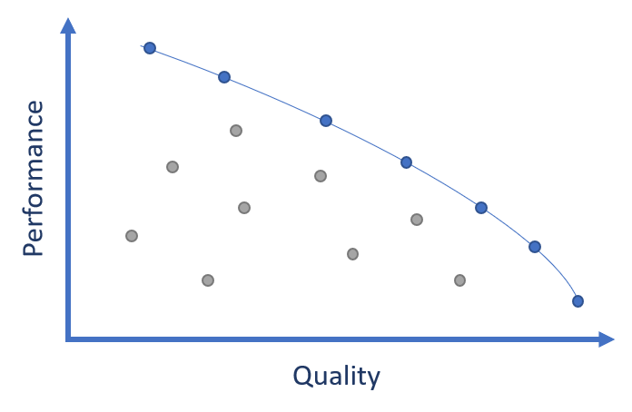
Any compressor that falls behind the frontier - the grey points in the figure above - is effectively obsolete. A user should be choosing an alternative which gives more quality at the same performance, or more performance at the same quality.

Pareto optimizations

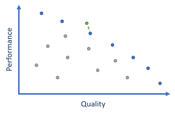
When optimizing a lossy compressor we don’t need to keep identical image output because the user isn’t expecting a specific output bit pattern anyway. The only hard requirement is that the changes give a net improvement relative to the existing frontier.

We have found many parts of the codec that do not justify their runtime cost. Removing these gives an absolute drop in image quality for that specific configuration, but moves the optimized codec to a new state-of-the-art position on the Pareto frontier.

While this seems like a loss for image quality, it is important to remember that this isn’t a zero-sum game. With a highly configurable compressor like astcenc we can increase the search depth elsewhere, and as long as that is less expensive than the performance the optimization gained, the overall frontier advances.

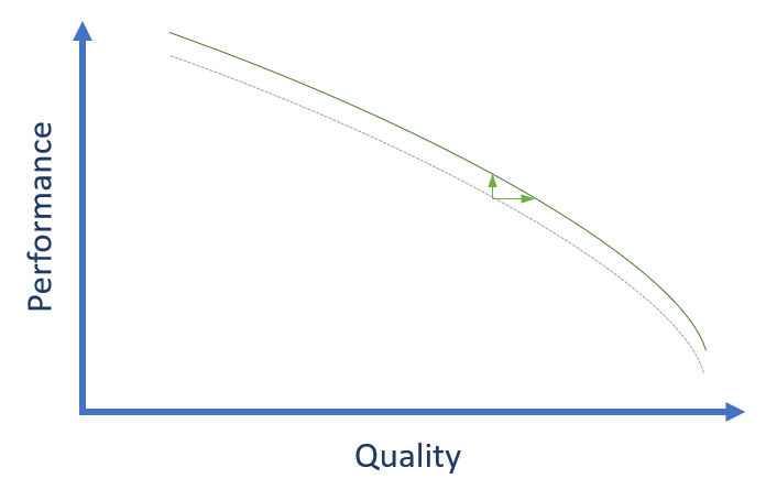
The only case where this argument isn’t true is for the highest quality configuration. If we remove options that impact the best quality mode there isn’t a “better quality” option that can be used to recover any quality losses. We are therefore more careful with search-space reductions that impact the high quality modes, as that is quality permanently lost to the void.

Optimizing along the frontier

Most of the optimizations to the compressor have been about trying to manage the amount of encoding space that is searched during compression. Intelligently reducing the search space is direct performance win, as the compressor needs to do much less work testing encodings for suitability.

However, the downside is that heuristics that cull search space are never perfect. We will sometimes guess wrong and skip encodings that would have given a better result. As long as the quality loss is sufficiently low that we end up on the right side of the Pareto frontier, then these have usually proven to be good changes to make.

Static search space reduction

The biggest changes I made to the compressor were those that simply removed portions ASTC encoding space from consideration. There are valid encodings that the compressor is now simply incapable of generating, because they are so rarely useful in practice that it’s not worth testing them.

ASTC allows two planes of weights for two and three partition encodings, but trying to store this many weights and four or six color endpoints nearly always requires too much quantization of the stored values to be useful. Therefore astcenc now only support two planes of weights for one partition encodings, removing a significant amount of the search space.

A bonus side-effect of this removal is that the multi-partition paths in the codec now only have to handle a single weight plane. This allows a significant simplification of this code path, which gives us improved performance for multi-partition searches.

Dynamic search pace reduction

The second set of changes I made to the compressor were those that dynamically reduce the search-space based on predicted benefit of those encodings. This is mostly based on data point extrapolation from earlier encodings. Do some trials, and based on that empirical data extrapolate to see if further trials along that axis are likely to beat the best encoding that we already know about.

We apply this to the use of two planes of weights. ASTC can assign any one of the color channels to the second weight plane, so we have 4 candidates to try for RGBA data. If the error for the first attempted dual-plane encoding is more than X% worse than best single-plane encoding, then we assume that no dual-plane encoding is worth considering and early-out the dual-plane searches.

We can be quite conservative with the values of X here. A lack of bitrate means that image quality often collapses for bad coding choices. Conservative thresholds such as “skip if 2x worse than current best encoding” are relatively safe but still manage to prune a significant number of searches.

We also apply this to the use of multiple color partitions. If the N+1 partition encoding is more than X% worse than the best N partition encoding, then we stop the search and don’t even try N+2. Again, we can be quite conservative on the thresholds to avoid hurting quality and still manage to cull a lot of trials.

The X values of the cut-off thresholds are determined by the current compressor quality profile. We get fine control over the heuristics, and can still allow the highest search qualities to test a significant portion of the search space.

There is probably more opportunity here for compressor innovation to make better up-front predictions without the initial trials, but that’s for the future …

Predictive extrapolation

Texture compression is mostly about making a good initial guess and then applying iterative refinement to jiggle colors and weights around to improve the final result. That iterative refinement is critical to getting a good quality output, as quantized errors are hard to predict, but can be very expensive.

Within each encoding trial we apply a predictive cull to the iterative refinement of colors and weights. We know, based on offline empirical analysis of many textures, how much iterative refinement is likely to improve block error. It’s around 10% for the first refinement pass, and 5% for the second pass, and 2% for the third.

To reduce the number of useless iterations we estimate, based on the number of iterations remaining, whether a block is likely to beat the current best block. If it’s not going to intersect then we simply stop and move on to the next candidate. This is a remarkably effective technique! Most candidate encodings early out and, on average, we only run 10% of the refinement passes for medium quality searches.

Code optimization

This section of the blog is not about ASTC specifics at all, but more about general software optimization techniques that I found worked well.

Vectorization

The first tool in the toolbox for any data crunching workload has to be trying to apply vectorization to the problem. The biggest challenge with modern SIMD is trying to have a solution that is flexible enough to handle the range of SIMD implementations that users will want to target without drowning in a maintenance headache of per-architecture implementations for every algorithm.

Most modern compilers seem to do a relatively good job with intrinsics, so the approach taken for astcenc is a light-weight vector library with vfloat, vint and vmask classes that wrap the platform-specific intrinsics. The underlying classes are explicit length (e.g. vfloat4, vfloat8), but we set up a generic (e.g. vfloat) typedef mapped to the longest length available for the current target architecture. This allows the core of the codec to be written using length-agnostic types, so it transparently handles the switch to AVX2, or Arm SVE2 in future. I am eternally grateful to @aras_p for the PR contribution of this library - it has been a fantastic tool in the toolbox.

It is worth noting that there are a few places where keeping things cross-platform does cost some performance, because x86 and Arm do have some minor differences which the library has to abstract away. One example of this is the vector select operation; x86-64 vblend uses the top bit in each lane to select which input register is used for the whole lane, whereas Arm NEON bsl simply does a bit-wise select so needs all bits in the lane set to 1.

AoS to SoA data layout

Effective vectorization needs a lot of data in an easy-to-access stream layout so you don’t waste cycles unpacking data. A heavy pivot to structure-of-array data layouts is needed, giving you efficient contiguous streams of data to operate on.

This does come with a downside unfortunately, which is register pressure.

The original AoS vector code might have been operating on a nice vfloat4 of RGBA data, which uses one SIMD register. Switch that into AoS form and we now have a vfloat of RRRR, GGGG, BBBB, and AAAA. 4 registers just for the input data. With SSE and AVX2 having just 16 vector registers to play with, things can get tight very quickly, especially if you need long-lived variables that persist across loop iterations such as per component accumulators.

One advantage of SoA is that it’s easier to skip lanes. It is common to have RGB data without an alpha channel so using SoA-form means we can simply omit the alpha vector from the calculation. Doing this for the original AoS form would just give a partial vector, and does not give any speedup.

Vectorized loop tails

When vectorizing data paths you need to work out how to handle any loop tail. You can include a scalar loop to clean up the loop tail but with loops that only have tens of iterations, which is common in ASTC, the scalar loop tail can end up being a significant percentage of the overall cost.

A much better design is to simply design the algorithm to allow the vectorized loop to include the loop tail. Where possible, round up arrays to a multiple of SIMD size and fill the tail with values which have no impact on the processing being performed. This might mean filling the tail with zeros, or it might mean replicating the last value. It depends on what you are doing.

If you cannot make the tail padding passive to the algorithm, you’ll need to start proactively managing the tail and masking lanes. Ideally you can do this outside of the main loop, but in the worst-case you need to add lane masking into the main loop. This starts to cost performance due to the added mask operations, and the register pressure of the masks themselves. However, for most short loops in astcenc this is usually still faster than a separate scalar tail loop.

Branches

Modern processors only like branches that they are able to predict. Failing to predict a branch correctly can result in 10+ cycle stall while the processor unpicks the bad guess and refills the pipeline. It doesn’t take many bad predictions for that kind of stall to hurt performance.

Compressor encoding decisions based on the data stream usually end up close to random, as data blocks rarely repeat the same pattern. Branches for these data-centric coding decisions are inherently unpredictable, so half the time you hit them you will pay the misprediction penalty.

The fix here is relatively simple - ban data-dependent branches in the critical parts of the the codec unless they are branching over a lot of work. For small branch paths simply compute both paths and use a SIMD select instruction to pick the result you want.

This can get a little untidy if you are selecting scalar variables. There is some overhead to packing scalar values into vector types so you can run select on them, but even with this messing about it’s still normally a net-win given the high cost of the mispredictions.

Specialization

Generic code is often slow code with a lot of control flow overhead to handle the various options that the generic path supports. One useful technique is specializing functions for commonly used patterns, and then selecting which function variant to run based on the current operation in hand. This is effectively a form of manual loop hoisting - pulling decisions up to an earlier point in the stack.

This has an overhead in terms of performance, as you will have higher instruction cache pressure due to the larger code size, so the gain from specialization needs to be higher than the loss due to cache misses.

In addition, developers will have a higher future maintenance cost to handle as there are now multiple variants to test and maintain. Therefore, only apply this technique where the specialization provides a significant reduction in code path complexity and is used with relatively high frequency.

For astcenc there are two main specializations that are used widely throughout the codec:

• Separate compressor passes for 1 and 2 weight planes.
• Separate compressor passes undecimated (1 weight per texel) and decimated (less than 1 weight per texel) weight handling.

… but there are many other more localized examples in the code.

Data table compaction

Caches matter. TLBs matter. If your algorithm churns your cache then your performance will take a massive hit. A L1 miss that hits in L2 takes ~20 cycles to resolve, and L2 miss may take 100 cycles …

There are a whole collection of techniques here, but there are three I’ve found most useful.

The compressor uses a lot of procedurally generated tables for partitioning and weight grid decimation information. Due to the way the ASTC header and partitioning schemes are encoded, many of the possible entries in the tables are not needed. Many entries are not useful (degenerate, duplicates, or disabled in the current compressor configuration). The original compressor stored things in encoding order, allowing direct indexing but requiring iteration through these unused values.

The codec now repacks the data tables to tightly pack the active entries, ensuring we only iterate through the useful data.

Splitting structures can also be a good technique. Different parts of the codec need different bits of the generated tables, and if it’s all interleaved in a single structure you often pollute the cache pulling in bits you don’t currently need. Splitting structures into tightly packed temporally-related streams helps to reduce the amount of collateral damage on your caches.

The final change is type size reduction. Narrow types in memory = less cache pressure = more performance. The one gotcha I’ve hit with this is that the AVX2 gather operations only support 32-bit accesses, so there are cases where we could have used narrower types but were forced to promote to 32-bit so we could use hardware gathers.

Deabstraction

Code with nicely modular functionality with clean interfaces and a high degree of orthogonality is great for maintainability and legibility. But it can be terrible for performance. The main pain-point is that you typically need to round-trip data via memory when crossing layers in the abstraction, so you end up spending a lot of time picking up and putting down data rather that actually doing useful processing.

Tactically removing abstractions on critical paths, and merging loops so we only have to touch data once, can be a very powerful tool. BUT, remember that you are probably making your code less maintainable so only do this where it makes a significant difference.

Link-time optimization

Modern compilers support link-time optimization, which effectively allows code generation to optimize across files (translation units). I found this gave a 5-10% performance boost for almost zero effort, and gave a 15% code size reduction for the core library.

Early LTO had a bad reputation for codegen reliability, but I’ve not had any problems with it, so give it a go.

One side-effect of LTO is that manually applying “classical” optimizations, such as improving function parameter passing to align with ABI requirements, often doesn’t help because LTO has already optimized away the inefficiency. Helpful, but frustrating when you think you’re on to a winner than winds up not actually helping …

Code deoptimization

A lot of optimization work turns into trying things that turn out not to help, or which don’t justify their complexity. Knowing what didn’t work is probably just as useful as knowing what worked …

Decrementing loops

An old trick on the early Arm CPUs I started programming on was to use decrementing loops, which use zero as a terminator condition. The idea here was that compare with zero is less expensive than a compare with a non-zero value. I didn’t really expect this to help on modern hardware, and it didn’t …

Approximate SIMD reciprocals

The SSE instruction set includes some operations to compute approximations of the reciprocal and the reciprocal square root of a number. On some late 1990s hardware these were worth using, as the real division was probably a scalar loop over the vector, but on modern hardware they are almost never a gain.

The first performance problem is that these estimates are not actually that accurate. Unless you can use the initial estimate directly, you will need to add at least one iteration of Newton-Raphson in to improve the accuracy which makes the operation a lot more expensive.

The other performance problem is that you replace SIMD divides (which execute in a dedicated divisor pipeline) with instructions which operate in the general purpose SIMD processing pipelines. The “expensive” division operation is effectively free as long as you can hide the result latency, whereas the “fast” alternative clogs up the functional units you really wanted to be using to do other work.

The final problem is a functional one. We want invariant output by default, and these instructions produce variable results across vendors and across products from the same vendor.

Consign these intrinsics to the history books - they have no place in new code.

Vectorizing long loops

There are two functions in the top ten list that are only 30% vectorized, both of which have relatively long loop bodies with a large number of live variables. I’ve tried numerous times to vectorize these functions with SoA, but end up with something that is slightly slower than what I already have. This is a classic example of SoA form increasing register pressure, and 16 vector registers just not being enough to hold the state of the program.

In some cases splitting loops can be helpful - two smaller loops run serially can mitigate register pressure issues - but you usually need to duplicate some memory loads or some computation that would have previously been shared - so I’ve found this very hit-and-miss.

Wide vectorization

Optimizing for AVX2 gives us access to 8-wide vectors, which we typically use to target using SoA memory layout so we can write vector-length agnostic code. When vectorizing in this form we’re often trying to replace code which is already vectorized 4-wide using AoS RGBA vectors. This gives two challenges.

Firstly the available peak uplift is only 2x vs what we have already, which in the grand-scheme of things isn’t a particularly large multiplier. It’s very easy to “spend” this gain on overhead if you need to start adding lane masking or other forms of sparse data/loop tail management.

The other challenge is that we also still need to maintain the performance of 4-wide SSE and NEON. For these use cases we can accept no improvement, but we really don’t want a regression with the new solution.

There are definitely parts of the code where using 8-wide vectors has proven beyond my abilities to achieve a net gain in performance for AVX2, let alone the fallback case.

Compacting variably-sparse memory

ASTC uses a lot of data tables, and for the most part we store these as fixed-size structures which contain enough space for the worst-case texel count, partition count, and weight count. Nearly every structure entry contains a considerable amount of padding, because the worst case is rare.

I tried shrinking these to store only what each case needed to improve memory locality. However, because the compaction is different in every case you inevitably need to start storing some additional level of indirection - either an actual pointer or an array offset for a packed array. Suddenly you put a dependent memory lookup on your critical path, so any gain is lost. Direct addressing is really useful and painful to lose.

Useful tools

Serious optimization needs profiling so you know where to focus effort. I use a variety of profilers, depending on what I’m trying to do.

I will profile release builds but with LTO turned off; it just makes too much of a mess of the data. Just be aware that you’re not entirely profiling reality. The compressor uses a lot of inlined functions, so I will selectively disable inlining by manually tagging interesting functions on the call path I’m looking at with “__attribute__((noinline))”. Without this, you just see all the time in the first non-inlined function which is often not all that useful.

Valgrind’s callgrind profiler is a good place to start - it’s easy to use. There are also some nice tools to generate annotated call graph diagrams from the output. which can help you pin down why some functions are being called a lot. The one gotcha with callgrind is that the default profile is based on instruction counts, which don’t always exactly align with wall-clock runtime, but it does have the advantage that it’s free of noise.

For micro-architecture profiling I use hotspot profilers such as the Linux Perf tools, or the Arm Streamline tool (declaration - I work on Streamline), both of which can be augmented with CPU performance counter feedback. The hotspot profiling gives you low-overhead mechanisms to identify where the time is spent and the counter feedback helps to explain why (cache misses, branch mispredicts, lack of vectorization. etc).

One must have skill is a willingness to read disassembly. I rarely write assembler now - intrinsics are (usually) “good enough” with the latest compilers - but being able to check that the compiler is doing a good job is an essential skill. As always godbolt.org is a great tool for checking multiple compilers and architectures quickly.

Summary

This blog outlines the major highlights. I’m sure I’ve forgotten to include something, so I’ll keep this up to date with other tips and tricks that I think of in future.

Don’t be afraid to try things - refactoring code and moving things around often triggers some flash of insight even if the original reason for doing the change turns out to be a dud!

I hope you find this a useful source of inspiration! I have - just by writing this down I’ve thought of a few new ideas to try …

Follow ups

Update: I realised while writing this blog that the NEON emulation of the vblend “test MSB for lane select” behavior was probably unnecessary most of the time. The original NEON implementation was just a port of the existing 4-wide SSE library and inherited the same semantics, so I automatically added MSB replication to select() so we had the same behavior for all instruction sets. However …

For both x86 and NEON using SIMD condition tests will set all bits in the lane, so in these cases NEON doesn’t need to do MSB replication. Removing this saves two NEON instructions for every select(), and accounts for more than 95% of the select() instances in the codec. SIMD selects are used a lot in our hot loops, so improving NEON select() improved performance by almost 30%!

The one case where we rely on the MSB select behavior is for selecting float lanes based on their sign bit, so I added an explicit select_msb() variant for this use case. This is more expensive on NEON, but we only use it in one place in the codec so it’s only a minor inconvenience.

Updates

• 23 Apr ‘22: Added a section on tools.
• 24 Apr ‘22: Added sections on deabstraction and compacting variably-sparse memory
• 26 Apr ‘22: Added section on wide vectorization.
• 30 Apr ‘22: Added section on approximate SIMD reciprocals, and the follow on about NEON select performance.